44 add or remove data labels in a chart

How to add data labels from different column in an Excel chart? Right click the data series in the chart, and select Add Data Labels > Add Data Labels from the context menu to add data labels. 2. Click any data label to select all data labels, and then click the specified data label to select it only in the chart. 3. Add / Move Data Labels in Charts - Excel & Google Sheets Add and Move Data Labels in Google Sheets Double Click Chart Select Customize under Chart Editor Select Series 4. Check Data Labels 5. Select which Position to move the data labels in comparison to the bars. Final Graph with Google Sheets After moving the dataset to the center, you can see the final graph has the data labels where we want.

Adding Data Labels to a Chart (Microsoft Word) - Tips.Net You can add data labels to your chart by following these steps: Select Chart Options from the Chart menu. Microsoft Graph displays the Chart Options dialog box. Make sure the Data Labels tab is selected. (See Figure 1.) Figure 1. The Data Labels tab of the Chart Options dialog box. Use the radio buttons to select the type of data label you want ...

Add or remove data labels in a chart

Edit titles or data labels in a chart - support.microsoft.com Right-click the data label, and then click Format Data Label or Format Data Labels. Click Label Options if it's not selected, and then select the Reset Label Text check box. Top of Page Reestablish a link to data on the worksheet On a chart, click the label that you want to link to a corresponding worksheet cell. Add vertical line to Excel chart: scatter plot, bar and line graph May 15, 2019 · Right-click anywhere in your scatter chart and choose Select Data… in the pop-up menu.; In the Select Data Source dialogue window, click the Add button under Legend Entries (Series):; In the Edit Series dialog box, do the following: . In the Series name box, type a name for the vertical line series, say Average.; In the Series X value box, select the independentx-value … Create Dynamic Chart Data Labels with Slicers - Excel Campus This is because Excel 2010 does not contain the Value from Cells feature. Jon Peltier has a great article with some workarounds for applying custom data labels. This includes using the XY Chart Labeler Add-in, which is a free download for Windows or Mac. Step 6: Setup the Pivot Table and Slicer. The final step is to make the data labels ...

Add or remove data labels in a chart. How To Add and Remove Legends In Excel Chart? - EDUCBA The data in a chart is organized with a combination of Series and Categories. Select the chart and choose filter then you will see the categories and series. Each legend key will represent a different color to differentiate from the other legend keys. Different Actions on Legends. Now we will create a small chart and perform different actions ... How to Add, Edit and Rename Data Labels in Excel Charts In this tutorial, you will learn how to add, edit and rename data labels in Microsoft excel graphs.#DataLabels #DataLabel #ExcelChart #ExcelGraph Add or remove titles in a chart To remove a chart title, on the Layout tab, in the Labels group, click Chart Title, and then click None. To remove an axis title, on the Layout tab, in the Labels group, click Axis Title, click the type of axis title that you want to remove, and then click None. To quickly remove a chart or axis title, click the title, and then press DELETE. Add or remove titles in a chart - support.microsoft.com Add or remove titles in a chart Article; Show or hide a chart legend or data table Article; Add or remove a secondary axis in a chart in Excel ... Under Labels, click Chart Title, and then click the one that you want. Select the text in the Chart Title box, and then type a chart title.

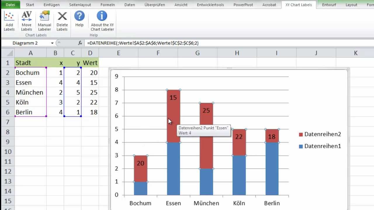
Add Totals to Stacked Bar Chart - Peltier Tech Oct 15, 2019 · Next, add data labels to the line chart series, above the points (below left). The default labels are Y values, so you don’t need to change anything. Finally, a little clean up. Hide the Totals line (format it to use ‘No Line’) and remove the Totals legend entry (click once on the legend, then a second time to select the legend entry, and ... Data Labels - IBM How to Remove Individual Data Labels You can remove the data labels if you no longer want to display them. If you are not in data label mode, from the menus choose: Elements > Data Label Mode Click a data label. The Chart Editor no longer displays the data value label. How to Remove All Data Labels You can also remove all data labels. How to Add Total Data Labels to the Excel Stacked Bar Chart Apr 03, 2013 · Step 4: Right click your new line chart and select “Add Data Labels” Step 5: Right click your new data labels and format them so that their label position is “Above”; also make the labels bold and increase the font size. Step 6: Right click the line, select “Format Data Series”; in the Line Color menu, select “No line” How to add data labels from different column in an Excel chart? This method will introduce a solution to add all data labels from a different column in an Excel chart at the same time. Please do as follows: 1. Right click the data series in the chart, and select Add Data Labels > Add Data Labels from the context menu to add data labels. 2.

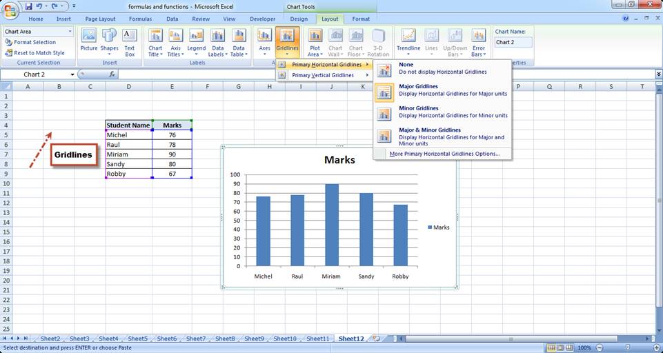
How to Add Gridlines in a Chart in Excel? 2 Easy Ways! So, a second way to add and format gridlines is to use the Design tab from the Chart Tools. Here’s how: Click on your chart. You should see the Chart Tools menu appear in the main menu. Select the Design tab from the Chart Tools menu. Click on ‘Add Chart Element’ (under the ‘Chart Layouts’ group). Add or remove data labels in a chart - support.microsoft.com Depending on what you want to highlight on a chart, you can add labels to one series, all the series (the whole chart), or one data point. Add data labels. You can add data labels to show the data point values from the Excel sheet in the chart. This step applies to Word for Mac only: On the View menu, click Print Layout. Data labels - Minitab Add data labels when you create a graph. You can add data labels to most Minitab graphs. In the dialog box for the graph you are creating, click Labels. Click the Data Labels tab or the tab for the specific type of data labels, for example Slice Labels, for pie charts. Choose the label options specific to the graph and click OK. Add & edit a chart or graph - Computer - Google Docs Editors … Double-click the chart you want to change. At the right, click Customize. Click Gridlines. Optional: If your chart has horizontal and vertical gridlines, next to "Apply to," choose the gridlines you want to change. Make changes to the gridlines. Tips: To hide gridlines but keep axis labels, use the same color for the gridlines and chart background.

Add data labels to a chart - Office Support

How to hide zero data labels in chart in Excel? - ExtendOffice In the Format Data Labelsdialog, Click Numberin left pane, then selectCustom from the Categorylist box, and type #""into the Format Codetext box, and click Addbutton to add it to Typelist box. See screenshot: 3. Click Closebutton to close the dialog. Then you can see all zero data labels are hidden.

Change the format of data labels in a chart

Create Dynamic Chart Data Labels with Slicers - Excel Campus Feb 10, 2016 · This is because Excel 2010 does not contain the Value from Cells feature. Jon Peltier has a great article with some workarounds for applying custom data labels. This includes using the XY Chart Labeler Add-in, which is a free download for Windows or Mac. Step 6: Setup the Pivot Table and Slicer. The final step is to make the data labels ...

Chart Types in PowerPoint

Clustered Column Chart in Power BI [With 45 Real Examples] Here we will see an example of the average line in a clustered column chart. Power BI clustered column chart average line. Expand the Average line, and select + Add line under the application settings to option. Once the line is added, Under the series, select the series for which you want to add a reference line.

Labels File - CHARTextract

Adding Data Labels to Your Chart (Microsoft Excel) To add data labels, follow these steps: Activate the chart by clicking on it, if necessary. Choose Chart Options from the Chart menu. Excel displays the Chart Options dialog box. Make sure the Data Labels tab is selected. (See Figure 1.) The left side of the dialog box shows the different types of data labels you can choose.

38 Add chart data labels - YouTube

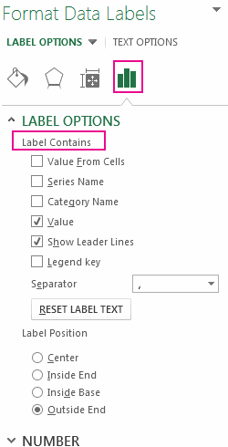
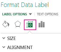
Change the format of data labels in a chart To get there, after adding your data labels, select the data label to format, and then click Chart Elements > Data Labels > More Options. To go to the appropriate area, click one of the four icons ( Fill & Line, Effects, Size & Properties ( Layout & Properties in Outlook or Word), or Label Options) shown here.

javascript - How to remove only one specific dataset label chartJS? - Stack Overflow

How to add or remove data labels with a click - Goodly Step 2) Place the dummy on the secondary axis Select the 2 data series (one by one) and use CTRL + 1 to open format data series box Then switch them to the secondary axis Note the secondary axis appears (we will hide that later) Step 3) Add data labels and fill the dummy with "no fill" Right click on the bar (dummy calculation) and add data labels

Excel - XY Chart Labeler - Diagramme beschriften - YouTube

Adding/Removing Data Labels in Charts - OzGrid After reading previous posts (particularly by norie and laplacian) I've decided that to remove a label from a single data point in a series on a chart I can't use the .HasDataLabels = false function, since it only applies to series objects. ... Adding/Removing Data Labels in Charts. Hi, The macro recorder yielded this syntax. [vba] ActiveChart ...

Chart's Data Series in Excel - Easy Excel Tutorial

How to add or move data labels in Excel chart? - ExtendOffice 1. Click the chart to show the Chart Elements button . 2. Then click the Chart Elements, and check Data Labels, then you can click the arrow to choose an option about the data labels in the sub menu. See screenshot: In Excel 2010 or 2007. 1. click on the chart to show the Layout tab in the Chart Tools group. See screenshot: 2.

Add Chart Labels – Grow Help Center

Show, Hide, and Format Mark Labels - Tableau Edit the label font: On the Marks card, click Label. In the dialog box that opens, under Label Appearance, click the Font drop-down. In the Font drop-down menu, you can do the following: Select a font type, size, and emphasis. Adjust the opacity of the labels by moving the slider at the bottom of the menu.

Basic Excel Chart Formatting - MS Excel Charting Tutorial Part 4 | Vertical Horizons

How to Add Data Labels to an Excel 2010 Chart - dummies Use the following steps to add data labels to series in a chart: Click anywhere on the chart that you want to modify. On the Chart Tools Layout tab, click the Data Labels button in the Labels group. None: The default choice; it means you don't want to display data labels. Center to position the data labels in the middle of each data point.

How do I supply my location label data? | Alltac Labels

Add or remove data labels in a chart - support.microsoft.com On the Design tab, in the Chart Layouts group, click Add Chart Element, choose Data Labels, and then click None. Click a data label one time to select all data labels in a data series or two times to select just one data label that you want to delete, and then press DELETE. Right-click a data label, and then click Delete.

Creating Pie Chart and Adding/Formatting Data Labels (Excel) - YouTube

Change axis labels in a chart in Office - support.microsoft.com The chart uses text from your source data for axis labels. To change the label, you can change the text in the source data. If you don't want to change the text of the source data, you can create label text just for the chart you're working on. In addition to changing the text of labels, you can also change their appearance by adjusting formats.

Use Google Forms to make a Pivot Chart - TechnoKids News and Blog Posts

How to Add Data Labels in Excel - Excelchat | Excelchat After inserting a chart in Excel 2010 and earlier versions we need to do the followings to add data labels to the chart; Click inside the chart area to display the Chart Tools. Figure 2. Chart Tools. Click on Layout tab of the Chart Tools. In Labels group, click on Data Labels and select the position to add labels to the chart.

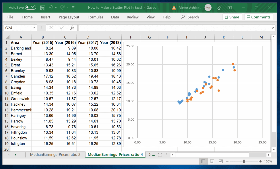
How to Make a Scatter Plot in Excel | Itechguides.com

Adding Data Labels to Charts/Graphs in Excel - Advantedge Training First Method - In the Design tab of the Chart Tools contextual tab, go to the Chart Layouts group on the far left side of the ribbon, and click Add Chart Element. In the drop-down menu, hover on Data Labels. This will cause a second drop-down menu to appear. Choose Outside End for now and note how it adds labels to the end of each pie portion.

How to create Custom Data Labels in Excel Charts – Efficiency 365

Adding Data Labels To An Excel Chart | MyExcelOnline In our example below, I add a Data Label to a column chart and then I format the data label using CTRL+1. I then select to custom format the numbers so it shows the values as thousands by adding a comma , after each zero and then showing the work k by adding "k" Example Custom Number Format: [$$-1004]#,##0 ,"k" ;- [$$-1004]#,##0 ,"k"

Excel 2013 Tutorial Formatting Data Labels Microsoft Training Lesson 28.6 - YouTube

how to add data labels into Excel graphs - storytelling with data To adjust the number formatting, navigate back to the Format Data Label menu and scroll to the Number section at the bottom. I'll choose Number in the Category drop-down and change Decimal places to 0 (side note: checking the Linked to source box is a good option if you want the labels to reformat when the formatting of the underlying source data changes).

Share :